Out-of-core analysis using Dask#
Author: Severin Dicks Copyright scverse
Here, we demonstrate the out-of-core computation capabilities of rapids-singlecell using Dask.
This approach allows us to analyze 1.3 million cells efficiently, even on relatively small hardware.
By leveraging Dask, we can:
Process large-scale single-cell datasets without exceeding memory limits.
Enable chunk-based execution, loading only the necessary data into memory at any time.
This method makes large-scale single-cell analysis feasible on standard hardware setups, removing barriers to working with massive datasets.
import dask
import time
import gc

from dask_cuda import LocalCUDACluster
from dask.distributed import Client
import rmm
import cupy as cp

from rmm.allocators.cupy import rmm_cupy_allocator
Initializing a Dask Cluster for Out-of-Core Computation#
To enable out-of-core computation and parallel processing, we initialize a Dask CUDA cluster, which distributes computations across available GPU resource.
Additional parameters for LocalCUDACluster#
CUDA_VISIBLE_DEVICES=preprocessing_gpus: selects GPUs to use (e.g.,
"0,1").threads_per_worker=10: CPU threads per GPU worker; tune for your workload and I/O.
protocol=”ucx”: enables UCX for high-throughput GPU-aware communication (NVLink/InfiniBand/RDMA).
rmm_pool_size=”10GB”: initial per-worker RAPIDS Memory Manager (RMM) pool; reduces allocation overhead.
rmm_maximum_pool_size=”20GB”: maximum pool growth per worker; allows RMM to expand up to this cap.
rmm_allocator_external_lib_list=”cupy”: integrates CuPy with RMM so CuPy allocations come from the pool.
Client(cluster): attaches the Dask client to the cluster (dashboard link available when running).
%%time
preprocessing_gpus="0,1"
cluster = LocalCUDACluster(CUDA_VISIBLE_DEVICES=preprocessing_gpus,
                           threads_per_worker=10,
                           protocol="ucx",
                           rmm_pool_size= "10GB",
                           rmm_maximum_pool_size = "20GB",
                           rmm_allocator_external_lib_list= "cupy",
                          )

client = Client(cluster)

client
CPU times: user 1.45 s, sys: 649 ms, total: 2.09 s
Wall time: 2.09 s
Client
Client-d167422f-bfc0-11f0-8f63-bcfce74fad1a
| Connection method: Cluster object | Cluster type: dask_cuda.LocalCUDACluster |
| Dashboard: http://127.0.0.1:8787/status |
Cluster Info
LocalCUDACluster
a9df7298
| Dashboard: http://127.0.0.1:8787/status | Workers: 2 |
| Total threads: 20 | Total memory: 503.20 GiB |
| Status: running | Using processes: True |
Scheduler Info
Scheduler
Scheduler-cb04d401-9edf-46e3-a42d-70fbe429f529
| Comm: ucx://127.0.0.1:48531 | Workers: 0 |
| Dashboard: http://127.0.0.1:8787/status | Total threads: 0 |
| Started: Just now | Total memory: 0 B |
Workers
Worker: 0
| Comm: ucx://127.0.0.1:47769 | Total threads: 10 |
| Dashboard: http://127.0.0.1:33327/status | Memory: 251.60 GiB |
| Nanny: ucx://127.0.0.1:33347 | |
| Local directory: /tmp/dask-scratch-space/worker-4__7tktz | |
Worker: 1
| Comm: ucx://127.0.0.1:37385 | Total threads: 10 |
| Dashboard: http://127.0.0.1:34947/status | Memory: 251.60 GiB |
| Nanny: ucx://127.0.0.1:58595 | |
| Local directory: /tmp/dask-scratch-space/worker-1bdf0brx | |
import rapids_singlecell as rsc
import scanpy as sc
import anndata as ad
Loading Large Datasets into AnnData with Dask#
To efficiently handle large-scale single-cell datasets, we load data directly from an HDF5 (h5) or Zarr file into an AnnData object using Dask arrays.
This enables lazy loading, allowing data to be processed in chunks without exceeding memory limits.
We achieve this using read_elem_as_dask, which loads the expression matrix (X) as a Dask array:
from importlib.metadata import version
from packaging.version import parse as parse_version
import zarr
if parse_version(version("anndata")) < parse_version("0.12.0rc1"):
    from anndata.experimental import read_elem_as_dask as read_dask
else:
    from anndata.experimental import read_elem_lazy as read_dask


SPARSE_CHUNK_SIZE = 20_000
#data_pth = "zarr/cell_atlas.zarr" #11 Million Cells
data_pth = "zarr/nvidia_1.3M.zarr" #1.3 Million Cells

f = zarr.open(data_pth, mode="r")
X = f["X"]
shape = X.attrs["shape"]
adata = ad.AnnData(
    X = read_dask(X, (SPARSE_CHUNK_SIZE, shape[1])),
    obs = ad.io.read_elem(f["obs"]),
    var = ad.io.read_elem(f["var"])
)
t1 = time.time()
rsc.get.anndata_to_GPU(adata)
Transferring AnnData to GPU for Accelerated Computation#
Once the dataset is loaded as a Dask-backed AnnData object,
we transfer it to the GPU to leverage RAPIDS-SingleCell’s accelerated processing.
We use rsc.get.anndata_to_GPU(), which efficiently moves the AnnData object to GPU memory:
Quality Control (QC) Metrics Calculation (Requires Synchronization)#
Before proceeding with further analysis, we compute quality control (QC) metrics
to assess dataset quality and filter out low-quality cells or genes.
We use rsc.pp.calculate_qc_metrics() to calculate key QC metrics
Although we are working with Dask-backed AnnData, this operation requires a synchronization step. This means that Dask computations must be evaluated immediately, so the process is not completely lazy like other out-of-core operations.
%%time
rsc.pp.calculate_qc_metrics(adata)
CPU times: user 6.64 s, sys: 727 ms, total: 7.37 s
Wall time: 7.35 s
Filtering Cells and Genes Without Additional Computation#
Instead of using sc.pp.filter_cells and sc.pp.filter_genes,
we apply filtering directly using boolean indexing to avoid extra computation.
Why Use Direct Indexing Instead of Built-in Functions?
More Efficient with Dask → Avoids triggering additional computations.
Preserves Lazy Execution → Filtering is applied without forcing full dataset evaluation.
Copy is preferred → Using
.copy()prevents views. Views slow down computations with Dask-backed AnnData.
adata = adata[(adata.obs["n_genes_by_counts"]<=10000)
            & (adata.obs["n_genes_by_counts"]>=200)].copy()
Log Normalization (Fully Lazy Execution)#
Next, we apply log normalization to scale gene expression values.
This step ensures that differences in sequencing depth across cells do not dominate downstream analysis.
%%time
rsc.pp.normalize_total(adata,target_sum = 10000)
rsc.pp.log1p(adata)
CPU times: user 5.73 ms, sys: 969 μs, total: 6.7 ms
Wall time: 4.95 ms
Selecting Highly Variable Genes (Requires Synchronization)#
To focus on the most informative features, we identify highly variable genes (HVGs)
using the Cell Ranger method and subset the dataset accordingly.
Important Considerations:
Requires Synchronization → Computing highly variable genes triggers evaluation, meaning this step is not fully lazy when using Dask.
Copy is preferred → Using
.copy()prevents views.
%%time
rsc.pp.highly_variable_genes(adata,n_top_genes=5000, flavor="cell_ranger")
adata = adata[:,adata.var.highly_variable].copy()
CPU times: user 5.58 s, sys: 479 ms, total: 6.05 s
Wall time: 6.04 s
Scaling Gene Expression (Requires Synchronization)#
To standardize gene expression values, we apply feature scaling,
ensuring that all genes contribute equally to downstream analysis.
Important Considerations:
Requires Synchronization → Since the input matrix is in CSR format (Compressed Sparse Row), this step forces an immediate computation, meaning it is not fully lazy like earlier transformations.
Scaling → Divides each gene’s expression values by its standard deviation.
zero_center=False → Keeps the scaled values non-centered, which is beneficial for sparse matrices and GPU acceleration.
%%time
rsc.pp.scale(adata, zero_center= False)
CPU times: user 5.56 s, sys: 462 ms, total: 6.02 s
Wall time: 6.01 s
Principal Component Analysis (PCA) on GPU (Two-Step Synchronization Process)#
To reduce dimensionality while preserving meaningful variation,
we perform Principal Component Analysis (PCA) using GPU acceleration.
Understanding the Two-Step Synchronization in PCA:
Mandatory Synchronization for Covariance & Mean Calculation
PCA requires computing the covariance matrix and mean vector, which must be explicitly synchronized before proceeding.
This step is handled automatically within
rsc.pp.pca().
Finalizing the Transformation with
.compute()After computing the principal components, the data remains lazy (Dask CuPy array).
Calling
.compute()onadata.obsm["X_pca"]performs the final transformation, projecting the data onto the computed PCs and materializing the result as a fully computed CuPy array.
Why This Matters?
The first synchronization (covariance & mean) ensures the PCA model is ready.
The second synchronization (
compute()) ensures that the transformed data is fully realized for downstream analyses like clustering and UMAP.
%%time
rsc.pp.pca(adata, n_comps = 100,mask_var=None)
adata.obsm["X_pca"]=adata.obsm["X_pca"].compute()
CPU times: user 12.9 s, sys: 1.75 s, total: 14.7 s
Wall time: 14.5 s
print(f"Time for the notebook: {time.time()-t1}s")
Time for the notebook: 34.43392086029053s
adata.obsm["X_pca"] = adata.obsm["X_pca"].get()
%%time
rsc.pp.neighbors(adata, n_neighbors=15, n_pcs=50, algorithm="ivfflat")
CPU times: user 2.02 s, sys: 318 ms, total: 2.33 s
Wall time: 2.13 s
%%time
rsc.tl.umap(adata)
CPU times: user 849 ms, sys: 169 ms, total: 1.02 s
Wall time: 798 ms
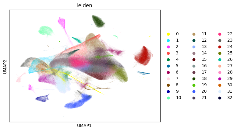
%%time
rsc.tl.leiden(adata)
CPU times: user 2.11 s, sys: 1.18 s, total: 3.29 s
Wall time: 2.86 s
sc.pl.umap(adata, color="leiden")