Squidpy-GPU

Accelerated Spatial Analysis

Author: Severin Dicks Copyright scverse

Here, we explore GPU-accelerated spatial analysis using rapids-singlecell’s rsc.gr module, which mirrors the API of Squidpy. We compute spatial autocorrelation metrics — Moran’s I and Geary’s C — to detect spatially structured genes within tissue sections.

By running these analyses on GPUs, we achieve faster computation and scalability for large spatial transcriptomics datasets, revealing biological patterns such as niche-specific expression and spatial gradients.

import squidpy as sq
import rapids_singlecell as rsc
import cupy as cp

import rmm
from rmm.allocators.cupy import rmm_cupy_allocator

rmm.reinitialize(
    managed_memory=False,  # Allows oversubscription
    pool_allocator=True,  # default is False
    devices=0,  # GPU device IDs to register. By default registers only GPU 0.
)
cp.cuda.set_allocator(rmm_cupy_allocator)

adata = sq.datasets.visium_hne_adata()

Constructing a Spatial Graph

Before computing spatial autocorrelation, we first need to build a spatial neighbors graph,
which defines spatial relationships between cells or tissue spots.

We use Squidpy to compute the graph based on spatial coordinates stored in adata.obsm["spatial"]

%%time
sq.gr.spatial_neighbors(adata)

CPU times: user 6 ms, sys: 89 μs, total: 6.08 ms
Wall time: 5.42 ms

genes = adata.var_names

Moran’s I

To assess spatial structure in gene expression, we compute spatial autocorrelation,
which measures how gene expression levels are spatially distributed across tissue sections.

%%time
rsc.gr.spatial_autocorr(adata, mode="moran", genes=genes, n_perms=100, use_sparse=False)

CPU times: user 396 ms, sys: 142 ms, total: 538 ms
Wall time: 533 ms

adata.uns["moranI"]

	I	pval_norm	var_norm	pval_z_sim	pval_sim	var_sim	pval_norm_fdr_bh	pval_z_sim_fdr_bh	pval_sim_fdr_bh
Nrgn	0.874753	0.000000	0.000131	0.000000	0.009901	0.000323	0.000000	0.000000	0.016667
Mbp	0.868723	0.000000	0.000131	0.000000	0.009901	0.000333	0.000000	0.000000	0.016667
Camk2n1	0.866545	0.000000	0.000131	0.000000	0.009901	0.000296	0.000000	0.000000	0.016667
Slc17a7	0.861761	0.000000	0.000131	0.000000	0.009901	0.000300	0.000000	0.000000	0.016667
Ttr	0.841988	0.000000	0.000131	0.000000	0.009901	0.000328	0.000000	0.000000	0.016667
...	...	...	...	...	...	...	...	...	...
Slc9a8	-0.026960	0.010027	0.000131	0.000327	0.009901	0.000066	0.017979	0.000610	0.016667
Pramef8	-0.028659	0.006681	0.000131	0.000011	0.009901	0.000043	0.012348	0.000024	0.016667
Klf12	-0.028764	0.006512	0.000131	0.000087	0.009901	0.000061	0.012052	0.000171	0.016667
Gart	-0.028859	0.006361	0.000131	0.000384	0.009901	0.000077	0.011784	0.000713	0.016667
Zbed4	-0.030420	0.004295	0.000131	0.000092	0.009901	0.000066	0.008154	0.000181	0.016667

18078 rows × 9 columns

Geary’s C

In addition to Moran’s I, we compute Geary’s C, another spatial autocorrelation metric.
While Moran’s I captures global spatial structure, Geary’s C is more sensitive to local differences,
highlighting regions with abrupt expression changes.

use_sparse=True Enables sparse computation, preventing full matrix densification. This optimization is handled efficiently in the GPU kernel, significantly reducing memory usage. Moran’s I also supports use_sparse=True, allowing for efficient computation on large datasets.

%%time
rsc.gr.spatial_autocorr(adata, mode="geary", genes=genes, n_perms=100, use_sparse=True)

CPU times: user 527 ms, sys: 40 ms, total: 567 ms
Wall time: 562 ms

adata.uns["gearyC"]

	C	pval_norm	var_norm	pval_z_sim	pval_sim	var_sim	pval_norm_fdr_bh	pval_z_sim_fdr_bh	pval_sim_fdr_bh
Nrgn	0.126481	0.000000e+00	0.000131	0.000000	0.009901	0.000337	0.000000e+00	0.000000	0.016733
Mbp	0.132854	0.000000e+00	0.000131	0.000000	0.009901	0.000300	0.000000e+00	0.000000	0.016733
Camk2n1	0.135106	0.000000e+00	0.000131	0.000000	0.009901	0.000322	0.000000e+00	0.000000	0.016733
Slc17a7	0.138819	0.000000e+00	0.000131	0.000000	0.009901	0.000322	0.000000e+00	0.000000	0.016733
Ttr	0.156155	0.000000e+00	0.000131	0.000000	0.009901	0.000343	0.000000e+00	0.000000	0.016733
...	...	...	...	...	...	...	...	...	...
AC166344.1	1.079271	2.059686e-12	0.000131	0.421383	0.049505	0.000050	7.064124e-12	0.436020	0.071936
Gm14091	1.083541	1.372236e-13	0.000131	0.424654	0.148515	0.001859	4.932845e-13	0.438104	0.189007
Slc6a5	1.087126	1.265654e-14	0.000131	0.447575	0.405941	0.000377	4.722497e-14	0.455640	0.428381
Soat2	1.093646	1.110223e-16	0.000131	0.436112	0.326733	0.000165	4.432556e-16	0.446482	0.361973
Bmp8b	1.125921	0.000000e+00	0.000131	0.385002	0.099010	0.000045	0.000000e+00	0.413767	0.133247

18078 rows × 9 columns

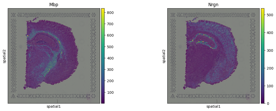
To explore spatial patterns in gene expression, we use Squidpy’s spatial scatter plot,
which overlays expression values onto the spatial coordinates of cells or tissue spots.

We visualize the expression of Mbp (myelin-associated) and Nrgn (neuronal marker):

sq.pl.spatial_scatter(adata, color=["Mbp", "Nrgn"])