Pearson Residuals Workflow

Author: Severin Dicks Copyright scverse

Here, we demonstrate the Pearson residuals workflow as an alternative to the standard log-normalization pipeline shown in 01_basic_workflow.ipynb. Pearson residuals provide variance-stabilized expression values that often improve highly variable gene selection and downstream analysis on sparse, heterogeneous single-cell datasets.

import warnings

warnings.filterwarnings("ignore")

import scanpy as sc
import cupy as cp

import time
import rapids_singlecell as rsc

import rmm
from rmm.allocators.cupy import rmm_cupy_allocator

rmm.reinitialize(
    managed_memory=False,  # Allows oversubscription
    pool_allocator=False,  # default is False
    devices=0,  # GPU device IDs to register. By default registers only GPU 0.
)
cp.cuda.set_allocator(rmm_cupy_allocator)

Load and Prepare Data

We load the sparse count matrix from an h5ad file using Scanpy. The sparse count matrix will then be placed on the GPU.

data_load_start = time.time()

%%time
adata = sc.read("h5/dli_census.h5ad")

CPU times: user 354 ms, sys: 1.36 s, total: 1.71 s
Wall time: 1.71 s

%%time
rsc.get.anndata_to_GPU(adata)

CPU times: user 158 ms, sys: 2.23 s, total: 2.38 s
Wall time: 2.38 s

data_load_time = time.time()
print("Total data load and format time: %s" % (data_load_time - data_load_start))

Total data load and format time: 4.109776496887207

Preprocessing

preprocess_start = time.time()

adata.var_names = adata.var.feature_name

Quality Control

We calculate quality control (QC) metrics to assess cell and gene quality. These include:

• Per cell metrics:

  • Total counts per cell (library size)

  • Number of detected genes per cell

  • Percentage of counts from mitochondrial (MT) and ribosomal (RIBO) genes

• Per gene metrics (gene space):

  • Total counts per gene

  • Number of cells expressing each gene

These metrics help identify low-quality or stressed cells and ensure a meaningful feature set for downstream analysis.

%%time
rsc.pp.flag_gene_family(adata, gene_family_name="MT", gene_family_prefix="MT")

CPU times: user 6.71 ms, sys: 0 ns, total: 6.71 ms
Wall time: 6.65 ms

%%time
rsc.pp.flag_gene_family(adata, gene_family_name="RIBO", gene_family_prefix="RPS")

CPU times: user 6.2 ms, sys: 103 μs, total: 6.31 ms
Wall time: 6.22 ms

%%time
rsc.pp.calculate_qc_metrics(adata, qc_vars=["MT", "RIBO"])

CPU times: user 70.1 ms, sys: 8.1 ms, total: 78.2 ms
Wall time: 77.7 ms

To visualize the quality control (QC) metrics, we generate the following plots:

1. Scatter plot: Total counts vs. Mitochondrial percentage

   • This plot shows the relationship between the total UMI counts per cell and the percentage of mitochondrial (MT) gene expression.

   • Cells with high mitochondrial percentages may indicate stressed or dying cells.

2. Scatter plot: Total counts vs. Number of detected genes

   • This plot displays the correlation between the total UMI counts per cell and the number of detected genes.

   • A strong correlation is expected, but outliers with low gene counts might indicate empty droplets or dead cells.

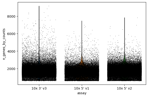
3. Violin plot: Number of detected genes per cell

   • This violin plot visualizes the distribution of the number of detected genes per cell.

   • It helps identify cells with abnormally low or high gene counts, which could be filtered out.

4. Violin plot: Total counts per cell

   • This plot shows the distribution of total counts per cell, indicating library size variation.

   • Extreme values may suggest low-quality or overly dominant cells.

5. Violin plot: Percentage of mitochondrial counts per cell

   • This plot illustrates the distribution of mitochondrial gene expression across all cells.

   • High mitochondrial content could be a sign of cell stress or apoptosis.

These visualizations help assess dataset quality and guide decisions on filtering low-quality cells.

sc.pl.scatter(adata, x="total_counts", y="pct_counts_MT")
sc.pl.scatter(adata, x="total_counts", y="n_genes_by_counts")

sc.pl.violin(adata, "n_genes_by_counts", jitter=0.4, groupby="assay")
sc.pl.violin(adata, "total_counts", jitter=0.4, groupby="assay")
sc.pl.violin(adata, "pct_counts_MT", jitter=0.4, groupby="assay")

Filter

We filter the count matrix to remove cells with an extreme number of genes expressed. We also filter out cells with a mitchondrial countent of more than 20%.

%%time
adata = adata[adata.obs["n_genes_by_counts"] < 5000]
adata = adata[adata.obs["pct_counts_MT"] < 20]

CPU times: user 128 ms, sys: 16.2 ms, total: 144 ms
Wall time: 143 ms

We also filter out genes that are expressed in less than 3 cells.

%%time
rsc.pp.filter_genes(adata, min_cells=3)

filtered out 33823 genes that are detected in less than 3 cells
CPU times: user 392 ms, sys: 101 ms, total: 493 ms
Wall time: 625 ms

The size of our count matrix is now reduced.

adata.shape

(213082, 28065)

Normalize

Before performing further transformations on the data, we store the raw count matrix in the .layers attribute.
This ensures that the original unnormalized expression values remain accessible for later analyses.

adata.layers["counts"] = adata.X.copy()

We normalize the count matrix so that the total counts in each cell sum to 1e4.

%%time
rsc.pp.normalize_total(adata, target_sum=1e4)

CPU times: user 1.78 ms, sys: 97 μs, total: 1.87 ms
Wall time: 1.41 ms

Next, we data transform the count matrix.

%%time
rsc.pp.log1p(adata)

CPU times: user 35.6 ms, sys: 19.1 ms, total: 54.6 ms
Wall time: 54.1 ms

adata.raw = adata

Identifying Highly Variable Genes

Next, we identify highly variable genes (HVGs), which capture the most biologically relevant variation in the dataset.
These genes are selected based on their variance, helping to reduce noise and focus on meaningful signals.

We use the Pearson residuals method to detect HVGs while preserving statistical robustness

%%time
rsc.pp.highly_variable_genes(
    adata, n_top_genes=5000, flavor="pearson_residuals", layer="counts"
)

CPU times: user 702 ms, sys: 60.5 ms, total: 762 ms
Wall time: 802 ms

Now we restrict our AnnData object to the highly variable genes.

%%time
rsc.pp.filter_highly_variable(adata)

CPU times: user 648 ms, sys: 400 ms, total: 1.05 s
Wall time: 1.27 s

adata.shape

(213082, 5000)

Normalize Pearson residuals

To correct for technical biases and overdispersion in single-cell data,
we apply Pearson residual normalization, a method that stabilizes variance across genes.

This transformation enhances the detection of biological variation while reducing noise.
We store the Pearson residuals in a separate layer to preserve the original data:

%%time
adata.layers["pearson_residuals"] = rsc.pp.normalize_pearson_residuals(
    adata, layer="counts", inplace=False
)

CPU times: user 152 ms, sys: 15 ms, total: 167 ms
Wall time: 167 ms

Performing PCA on Pearson Residuals

To reduce the dimensionality of the dataset while preserving meaningful variation,
we perform Principal Component Analysis (PCA) using the Pearson residuals.
This approach ensures that technical noise is minimized, allowing better downstream analysis.

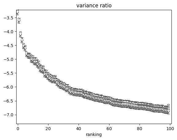
We compute 100 principal components (PCs) from the normalized data

%%time
rsc.pp.pca(adata, n_comps=100, layer="pearson_residuals")

CPU times: user 1.27 s, sys: 116 ms, total: 1.39 s
Wall time: 1.59 s

sc.pl.pca_variance_ratio(adata, log=True, n_pcs=100)

Now we move .X and .layers out of the GPU.

%%time
rsc.get.anndata_to_CPU(adata, convert_all=True)

CPU times: user 445 ms, sys: 324 ms, total: 769 ms
Wall time: 768 ms

preprocess_time = time.time()
print("Total Preprocessing time: %s" % (preprocess_time - preprocess_start))

Total Preprocessing time: 10.96704626083374

We have now finished the preprocessing of the data.