Pearson Residues Example

Author: Severin Dicks

To run this notebook please make sure you have a working rapids environment with all nessaray dependencies. Run the data_downloader notebook first to create the AnnData object we are working with. In this example workflow we’ll be looking at a dataset of 500000 brain cells from Nvidia.

import scanpy as sc
import cupy as cp

import time
import rapids_singlecell as rsc

import warnings

warnings.filterwarnings("ignore")

import rmm
from rmm.allocators.cupy import rmm_cupy_allocator

rmm.reinitialize(
    managed_memory=False,  # Allows oversubscription
    pool_allocator=False,  # default is False
    devices=0,  # GPU device IDs to register. By default registers only GPU 0.
)
cp.cuda.set_allocator(rmm_cupy_allocator)

Load and Prepare Data

We load the sparse count matrix from an h5ad file using Scanpy. The sparse count matrix will then be placed on the GPU.

data_load_start = time.time()

%%time
adata = sc.read("h5/500000.h5ad")
adata.var_names_make_unique()

CPU times: user 564 ms, sys: 2.52 s, total: 3.09 s
Wall time: 10.3 s

%%time
rsc.get.anndata_to_GPU(adata)

CPU times: user 414 ms, sys: 1.62 s, total: 2.04 s
Wall time: 2.04 s

Verify the shape of the resulting sparse matrix:

adata.shape

(500000, 27998)

And the number of non-zero values in the matrix:

data_load_time = time.time()
print("Total data load and format time: %s" % (data_load_time - data_load_start))

Total data load and format time: 12.361832857131958

Preprocessing

preprocess_start = time.time()

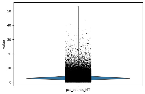
Quality Control

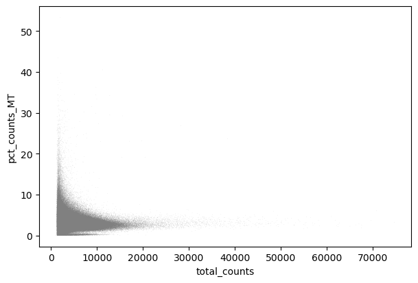
We perform a basic qulitiy control and plot the results

%%time
rsc.pp.flag_gene_family(adata, gene_family_name="MT", gene_family_prefix="mt-")

CPU times: user 5.41 ms, sys: 0 ns, total: 5.41 ms
Wall time: 5.29 ms

%%time
rsc.pp.calculate_qc_metrics(adata, qc_vars=["MT"])

CPU times: user 148 ms, sys: 9.6 ms, total: 158 ms
Wall time: 233 ms

sc.pl.scatter(adata, "total_counts", "pct_counts_MT")
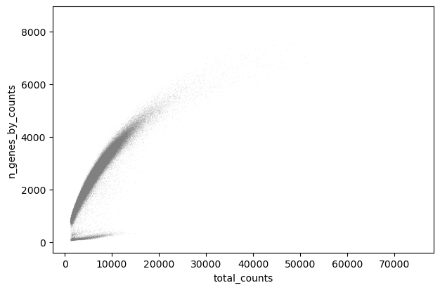
sc.pl.scatter(adata, "total_counts", "n_genes_by_counts")

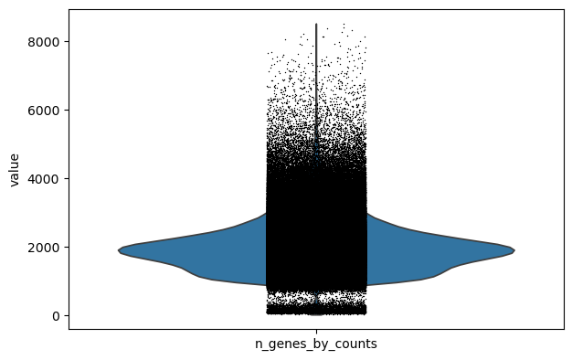
sc.pl.violin(adata, keys="n_genes_by_counts")
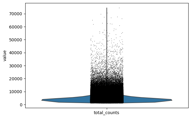
sc.pl.violin(adata, keys="total_counts")
sc.pl.violin(adata, keys="pct_counts_MT")

Filter

We filter the count matrix to remove cells with an extreme number of genes expressed. We also filter out cells with a mitchondrial countent of more than 20%.

The size of our count matrix is now reduced.

%%time
rsc.pp.filter_genes(adata, min_count=10)

filtered out 7663 genes based on n_cells_by_counts
CPU times: user 378 ms, sys: 42.2 ms, total: 421 ms
Wall time: 439 ms

%%time
rsc.pp.filter_cells(adata, qc_var="n_genes_by_counts", min_count=500, max_count=4000)
rsc.pp.filter_cells(adata, qc_var="total_counts", max_count=20000)
adata = adata[adata.obs["pct_counts_MT"] < 20]

filtered out 15844 cells
filtered out 5 cells
CPU times: user 139 ms, sys: 62.4 ms, total: 201 ms
Wall time: 765 ms

We copy the raw counts to the layer counts

adata.layers["counts"] = adata.X.copy()

Log-Normalize counts

We normalize the count matrix so that the total counts in each cell sum to 1e4.

%%time
rsc.pp.normalize_total(adata, target_sum=1e4)

CPU times: user 1.86 ms, sys: 692 µs, total: 2.55 ms
Wall time: 8.99 ms

Next, we log transform the count matrix.

%%time
rsc.pp.log1p(adata)

CPU times: user 30.2 ms, sys: 3.87 ms, total: 34.1 ms
Wall time: 50.9 ms

Now we safe this version of the AnnData as adata.raw.

%%time
adata.raw = adata

CPU times: user 666 ms, sys: 456 ms, total: 1.12 s
Wall time: 1.12 s

Select Most Variable Genes

Now we search for highly variable genes. This function only supports the flavors cell_ranger seurat seurat_v3 and pearson_residuals. As you can in scanpy you can filter based on cutoffs or select the top n cells. You can also use a batch_key to reduce batcheffects.

In this example we use pearson_residuals for selecting highly variable genes with .layers["counts"]

%%time
rsc.pp.highly_variable_genes(
    adata, n_top_genes=5000, flavor="pearson_residuals", layer="counts"
)

CPU times: user 3.01 s, sys: 67.7 ms, total: 3.08 s
Wall time: 3.15 s

Now we restrict our AnnData object to the highly variable genes.

%%time
rsc.pp.filter_highly_variable(adata)

CPU times: user 1.32 s, sys: 978 ms, total: 2.3 s
Wall time: 2.33 s

adata.shape

(483870, 5000)

Normalize

We normalize the raw counts matrix with pearson_residuals.

%%time
adata.layers["pearson_residuals"] = rsc.pp.normalize_pearson_residuals(
    adata, layer="counts", inplace=False
)

CPU times: user 974 ms, sys: 12.9 ms, total: 987 ms
Wall time: 1 s

Principal component analysis

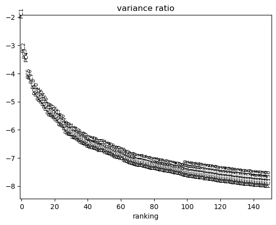
We use PCA to reduce the dimensionality of the matrix to its top 150 principal components. We use the PCA implementation from cuMLs.

We can use scanpy pca_variance_ratio plot to inspect the contribution of single PCs to the total variance in the data.

%%time
rsc.pp.pca(adata, n_comps=150, layer="pearson_residuals")

CPU times: user 2.58 s, sys: 110 ms, total: 2.69 s
Wall time: 3.28 s

sc.pl.pca_variance_ratio(adata, log=True, n_pcs=150)

Now we move .X and .layers out of the GPU.

%%time
rsc.get.anndata_to_CPU(adata, convert_all=True)

CPU times: user 1.07 s, sys: 988 ms, total: 2.06 s
Wall time: 2.06 s

preprocess_time = time.time()
print("Total Preprocessing time: %s" % (preprocess_time - preprocess_start))

Total Preprocessing time: 24.27028512954712

We have now finished the preprocessing of the data.

Clustering and Visualization

Computing the neighborhood graph and UMAP

Next we compute the neighborhood graph using rsc.

Scanpy CPU implementation of nearest neighbor uses an approximation, while the GPU version calculates the exact graph. Both methods are valid, but you might see differences.

%%time
rsc.pp.neighbors(adata, n_neighbors=15, n_pcs=60)

CPU times: user 4.92 s, sys: 94 ms, total: 5.02 s
Wall time: 5.04 s

Next we calculate the UMAP embedding using rapdis.

%%time
rsc.tl.umap(adata)

CPU times: user 1.22 s, sys: 71.9 ms, total: 1.29 s
Wall time: 1.29 s

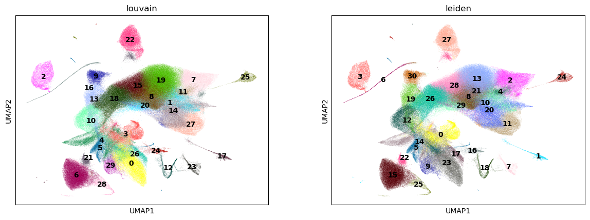
Clustering

Next, we use the Louvain and Leiden algorithm for graph-based clustering.

%%time
rsc.tl.louvain(adata, resolution=1.0)

CPU times: user 4.85 s, sys: 4.38 s, total: 9.24 s
Wall time: 11.1 s

%%time
rsc.tl.leiden(adata, resolution=1.0)

CPU times: user 1.51 s, sys: 3.62 s, total: 5.13 s
Wall time: 5.13 s

%%time
sc.pl.umap(adata, color=["louvain", "leiden"], legend_loc="on data")

CPU times: user 2.42 s, sys: 163 ms, total: 2.58 s
Wall time: 2.41 s

%%time
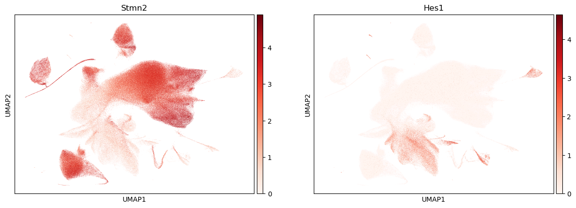
sc.pl.umap(adata, color=["Stmn2", "Hes1"], legend_loc="on data", cmap="Reds")

CPU times: user 3.33 s, sys: 162 ms, total: 3.49 s
Wall time: 3.32 s

%%time
rsc.tl.diffmap(adata)

CPU times: user 4.24 s, sys: 14.7 s, total: 18.9 s
Wall time: 1.7 s

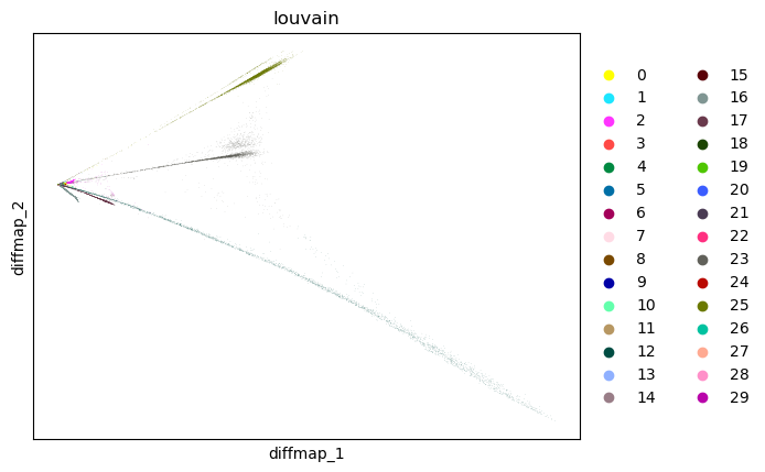
adata.obsm["X_diffmap_"] = adata.obsm["X_diffmap"][:, 1:]
sc.pl.embedding(adata, "diffmap_", color="louvain")

%%time
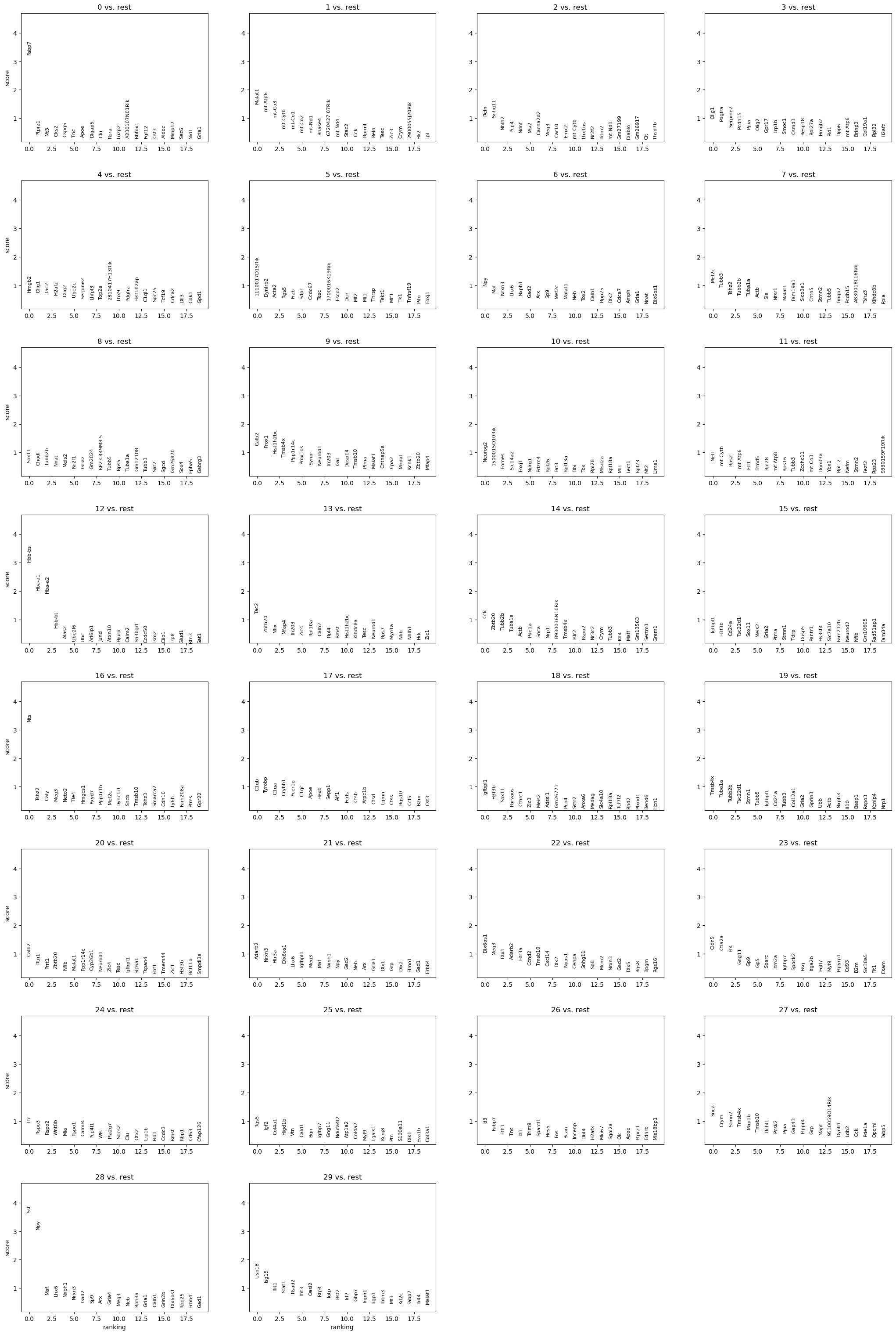
rsc.tl.rank_genes_groups_logreg(adata, groupby="louvain", use_raw=False)

[W] [17:00:21.909123] L-BFGS: max iterations reached
[W] [17:00:21.910102] Maximum iterations reached before solver is converged. To increase model accuracy you can increase the number of iterations (max_iter) or improve the scaling of the input data.
CPU times: user 1min 5s, sys: 3.42 s, total: 1min 9s
Wall time: 1min 9s

%%time
sc.pl.rank_genes_groups(adata, n_genes=20)

CPU times: user 2.8 s, sys: 225 ms, total: 3.03 s
Wall time: 2.85 s

print("Total Processing time: %s" % (time.time() - preprocess_start))

Total Processing time: 128.05585312843323